Just wait until you can see what you can do with a pivot table! No more tedious summarising of endless worksheets and data, the pivot table does it all for you.
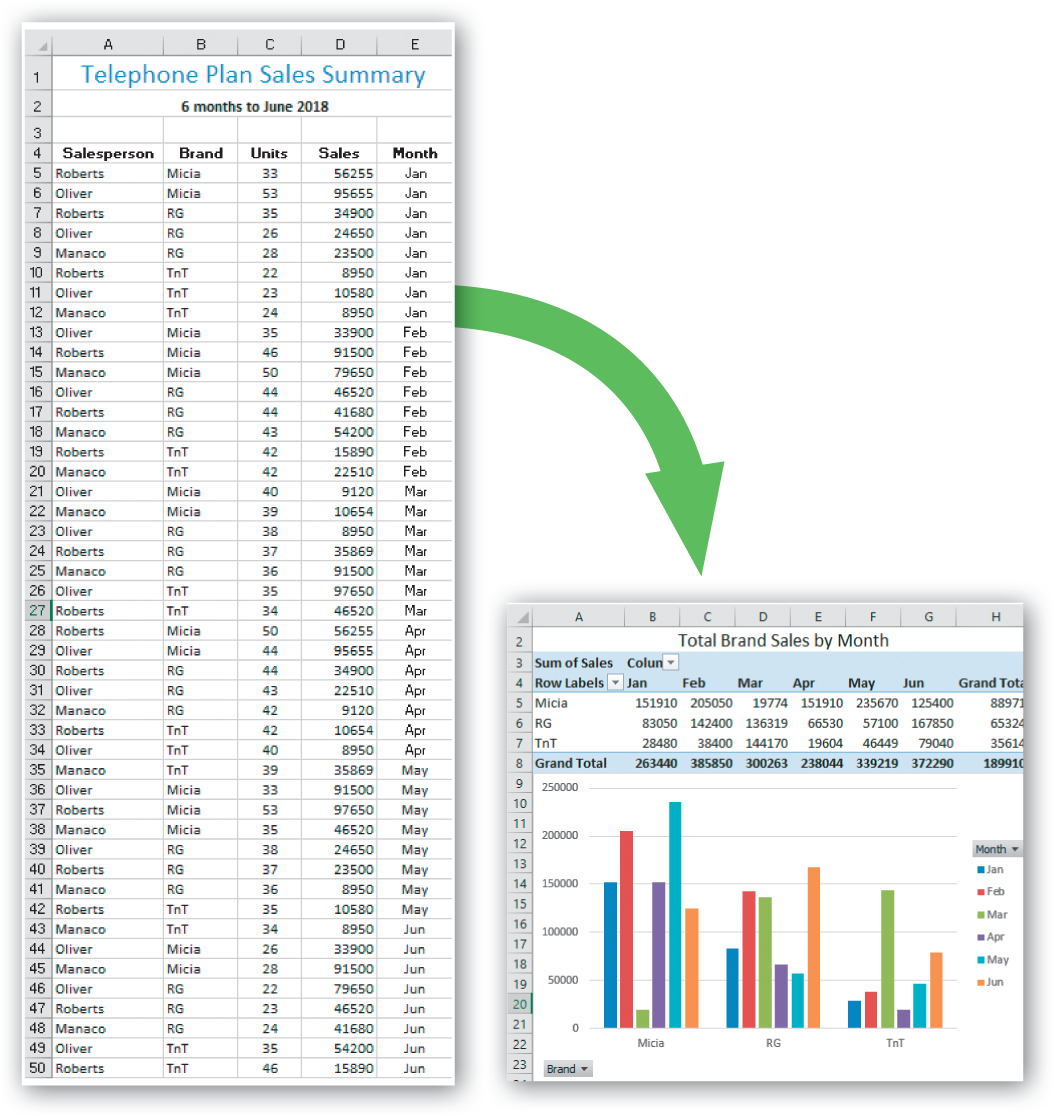
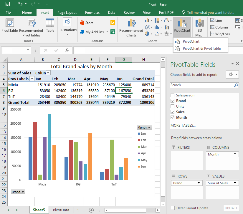
You can go from this list of data to this organised pivot table and pivot chart in seconds.
A pivot table is most useful when data within some of the columns is out of a few values (e.g. the product is one of three machines, the salesperson is either Owens, Phillips or Richards). The pivot table can be summarised easily around these distinctive categories.
Pivot tables work best with lists of data where there is a clear list of records with obvious headings as in the list above. The headings of each column are used to organise the data into a summary.
Open the Pivot workbook downloaded from the above link.
Select any cell in the list.
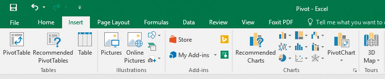
Click on the tab INSERT then the PIVOT TABLE button in the ribbon. For Google Sheets, click on DATA then PIVOT TABLE and then skip to step 7.
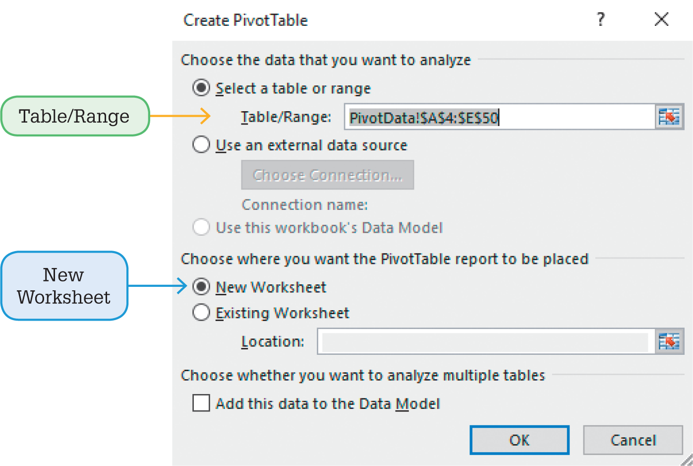
Check that the whole list is selected and the correct cell range is in the Table/Range box.
Check that NEW WORKSHEET is selected so the new pivot table is put into a separate worksheet.
Click on OK.
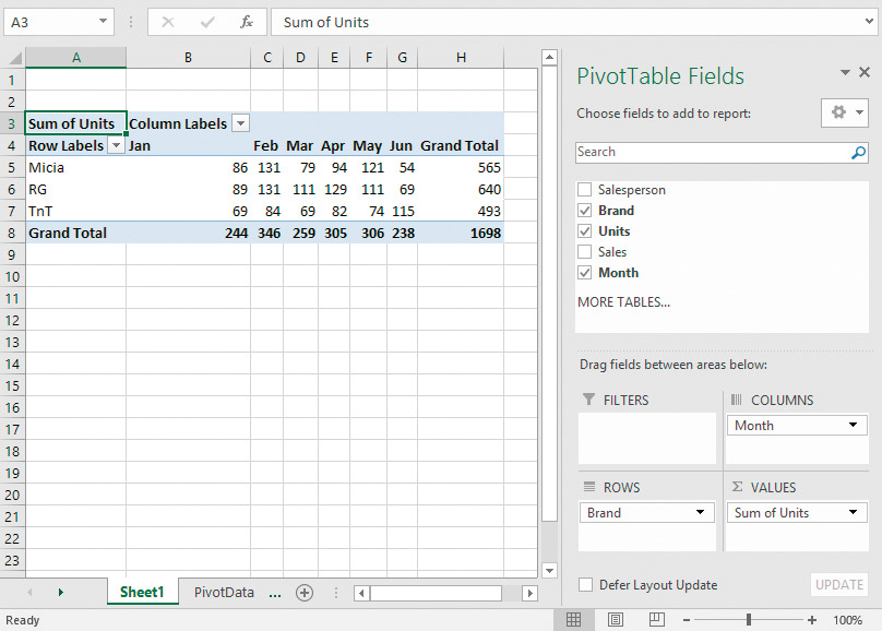
The new worksheet will be displayed and the pivot table task pane is opened as shown below. Notice that the task pane lists the fields from the original table. The lower part of the task pane is used to organise the structure of the pivot table. The pivot table task pane is only displayed while the active cell is within pivot table. The order you add fields to the structure determines the layout of the pivot table.
Click on the field BRAND, then MONTH – they will automatically be put in the ROWLABELS box. For Google Sheets, click on ADD FIELD for ROWS and select BRAND only.
Click on the field UNITS – it will automatically be put into SUM VALUES. For Google Sheets, click on ADD FIELD for VALUES and select UNITS.
Drag the MONTH field buttons over to the COLUMN LABELS box in the Task pane. For Google Sheets, click on ADD FIELD for COLUMNS and select MONTH. Your pivot table should appear as follows summarising the number of units sold for each product in each month.
Now to create another pivot table that summarises the monthly dollar value of sales by each salesperson for each brand.
Select the Pivot data worksheet to move back to the list.
Click on any cell in the list.
Click on the tab INSERT then the PIVOT TABLE button in the ribbon. For Google Sheets, click on DATA then PIVOT TABLE and skip to step 7.
Check that the whole list is selected and the correct cell range is in the Table/Range box.
Check that NEW WORKSHEET is selected so the new pivot table is put into a separate worksheet.
Click on OK.
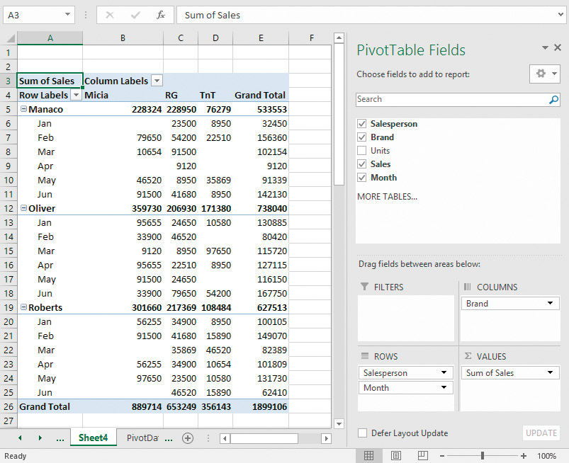
Click on the fields in this order: SALESPERSON, MONTH, BRAND – they will automatically be put in the ROW LABELS box. For Google Sheets, click on ADD FIELD for ROWS and select SALESPERSON and MONTH only.
Click on the field SALES – it will automatically be put into SUM VALUES. For Google Sheets, click on ADD FIELD for VALUES and select SALES.
Drag the BRAND field over to the COLUMN LABELS box. For Google Sheets, click on ADD FIELD for COLUMNS and select BRAND. Your table should appear as below.
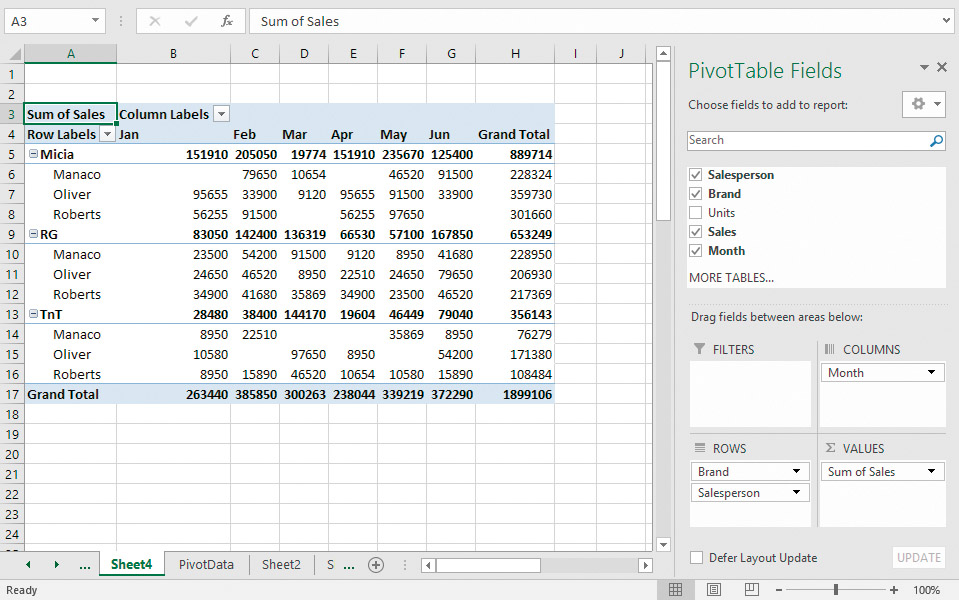
Drag the label for MONTH to the COLUMN LABELS box.
Drag the label for BRAND to appear before SALESPERSON. Now the data will be summarised by brand, then by salesperson for each month. Your pivot table should appear as follows.